2 Foundations of Probability
2.1 Introduction
The focus of this chapter is probability, and more specifically the theory of probability.
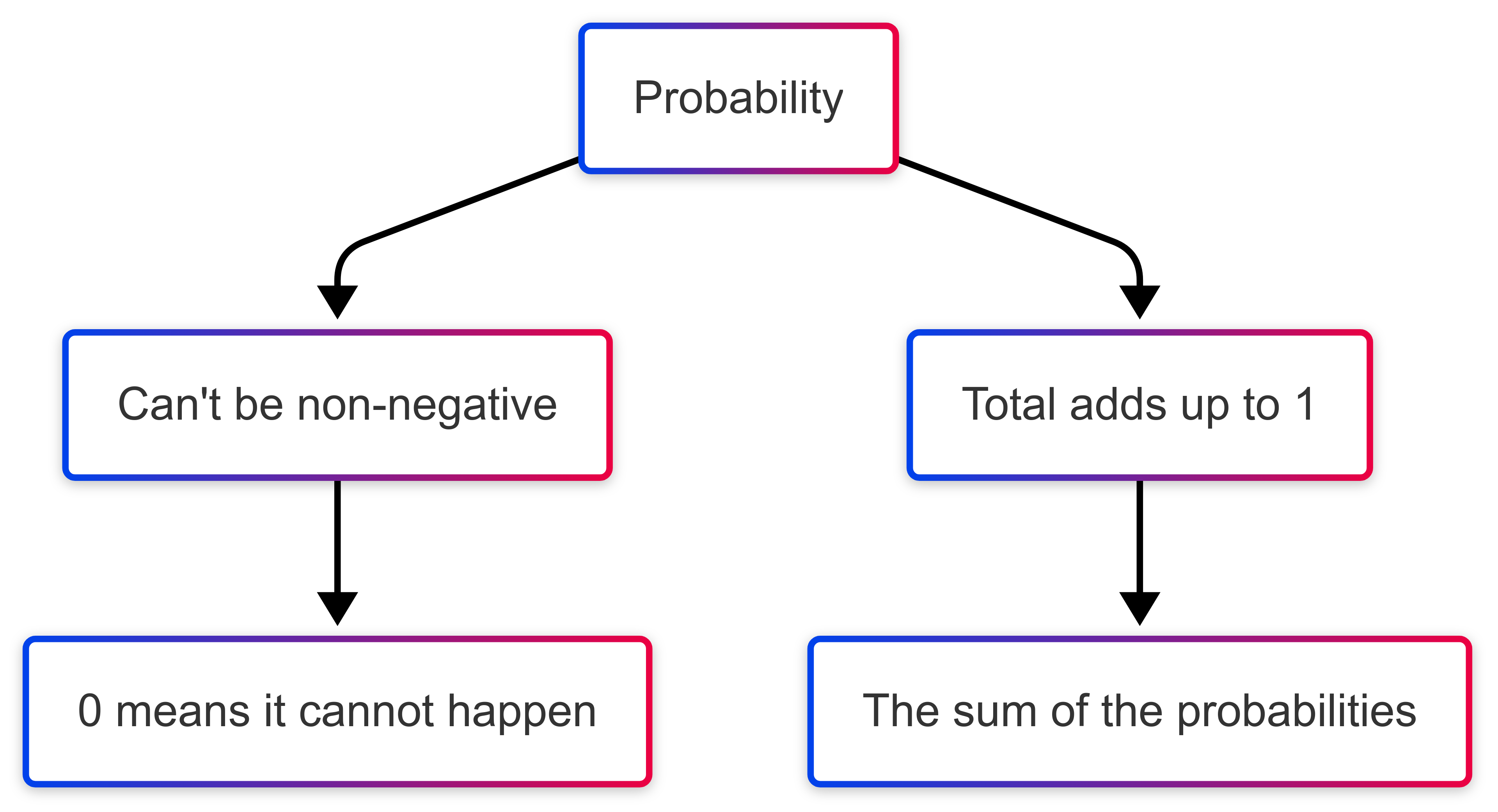
At its simplest,“probability is a measure of how likely an event is to occur. It’s expressed as a number between 0 and 1, where 0 means the event is impossible, and 1 means it is certain.
Definition
The study of probability is all about understanding and quantifying uncertainty [1].
Probability calculations define how likely outcomes are, modelled through probability spaces, the rules governing their interactions, and concepts such as conditional probability and independence.
Bayes’ Theorem, which we’ll cover at the end of the chapter, allows us to update probabilities based on new evidence.
Context
Probability emerged as a mathematical discipline in the 16th and 17th centuries, driven by questions arising from gambling and games of chance.
Mathematicians like Cardano, Fermat, and Pascal started to ask questions about practical problems of fairness and risk, leading to the formalisation of concepts such as ‘odds’ and ‘expected value’. You’ll still find these concepts, and probability more generally, at the heart of the sports betting industry today.
Notation
Discussions of probability often involve a number of special symbols. You’ll encounter the following in this chapter:
- \(∪\) (union) - represents “OR” between events
- \(∩\) (intersection) - represents “AND” between events
- \(P(A)\) - the probability of event A occurring
- \(P(A|B)\) - the probability of A given that B has occurred (conditional probability)
- Ac or A’ - the complement of A (event A does NOT occur)
- \(∅\) - an empty set (impossible event)
- \(Ω\) - pronounced ‘omega’, and represents the sample space (all possible outcomes)
2.2 Probability Spaces
Introduction
A ‘probability space’ is a mathematical construct that provides a formal framework for modelling random experiments and their outcomes.
Probability spaces give us a systematic way to analyse uncertainty and calculate probabilities in a rigorous manner.
Think of it as a complete mathematical description of a random process, like rolling dice or drawing cards, that captures all possible outcomes and their associated probabilities.
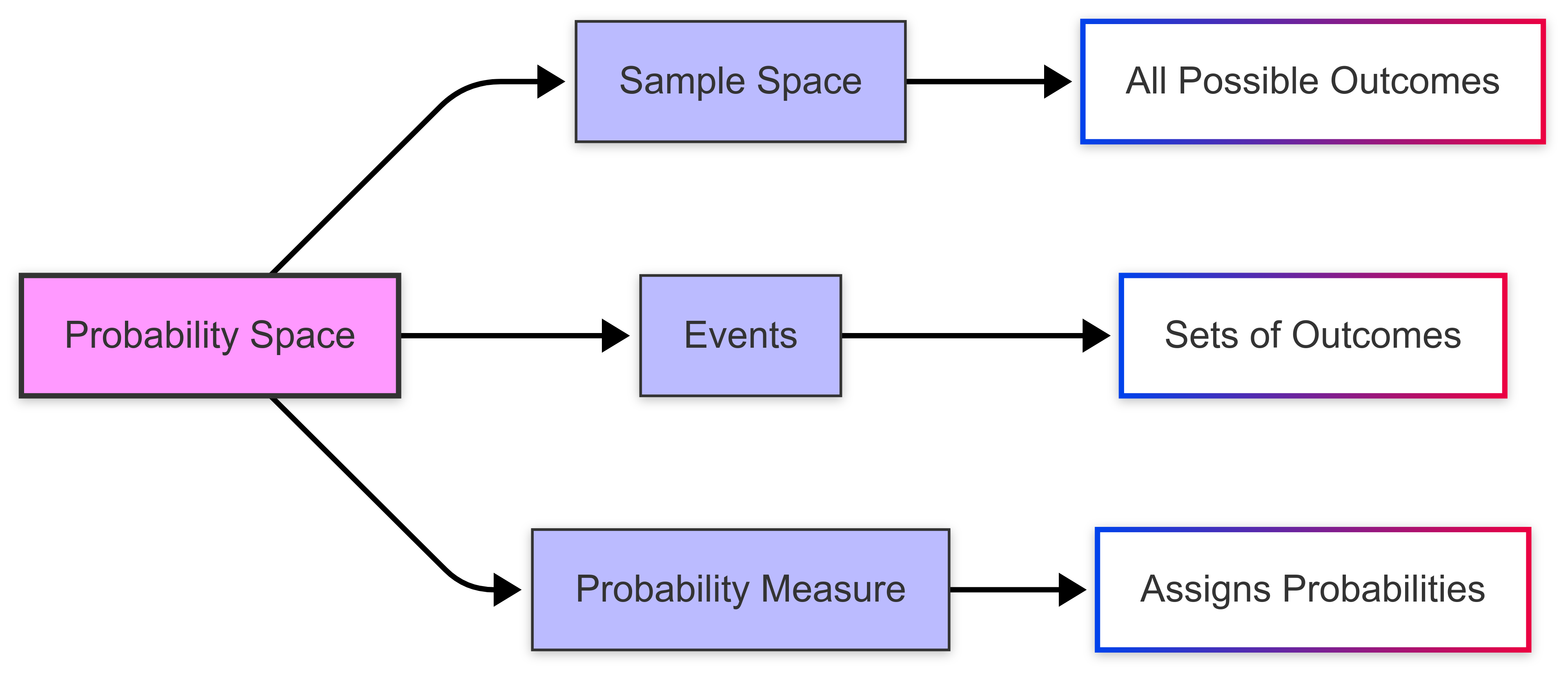
A probability space has three elements:
- a sample space;
- events; and
- a probability measure.
The probability space defines the structure for assigning probabilities to outcomes in an experiment.
What is the ‘sample space’?
The ‘sample space’ is the set of all possible outcomes in a random experiment.
For example, when flipping a coin, the sample space is {Heads, Tails}.
Each outcome in the sample space represents a result that could occur.
The sample space can be finite, like the roll of a die, or infinite, like measuring the exact time it takes for a task to complete.
The sample space gives us a foundation for defining events and calculating probabilities.
Some examples of sample spaces in sport include:
- Basketball shot: {Made basket, Missed shot}
- Tennis serve: {In, Out, Let, Fault}
- Football penalty kick: {Goal, Save, Miss}
- Golf shot: An infinite sample space representing the exact landing position coordinates of the ball
Note that sample spaces can vary from simple binary outcomes (win/loss) to complex sets of possibilities.
What are ‘events’?
In probability theory, an event is a specific set of outcomes from a sample space.
For example, when rolling a die, the event “rolling an even number” includes the outcomes {2, 4, 6}.
Events can involve a single outcome, like rolling a 3, or multiple outcomes, like rolling a number greater than 4.
Events are used to calculate probabilities by assigning a likelihood to the outcomes they contain.
Events in sport
In sport, events can be simple or complex:
- Simple events could include scoring a goal, making a basket, or hitting a home run
- Compound events could include winning a match, qualifying for playoffs, or breaking a record
For example, in football, the event “scoring from a penalty kick” has two possible outcomes: {success, failure}. More complex events like “winning the match” depend on multiple outcomes throughout the game.
2.3 How Do We Measure Probability?
A probability measure assigns a likelihood to events in a sample space.
Measuring probability follows three principles:
- probabilities are always non-negative;
- the probability of the entire sample space is 1; and
- the probabilities of mutually exclusive events add up. For example, in rolling a fair die, the probability measure assigns 1/6 to each outcome.
This measure allows us to calculate and compare the likelihood of different events.
Mathematically, we express probability as:
\[ P(A) = \frac{\text{Number of favorable outcomes}}{\text{Total number of possible outcomes}} \]
Where P(A) represents the probability of event A occurring. This formula applies when all outcomes are equally likely.
For example, when rolling a fair six-sided die, the probability of rolling a 3 is:
\[ P(\text{rolling a 3}) = \frac{1}{6} \]
Note that the sum of the probabilities of rolling a 1, 2, 3, 4, 5 or 6 totals 1.
2.4 The Rules of Probability
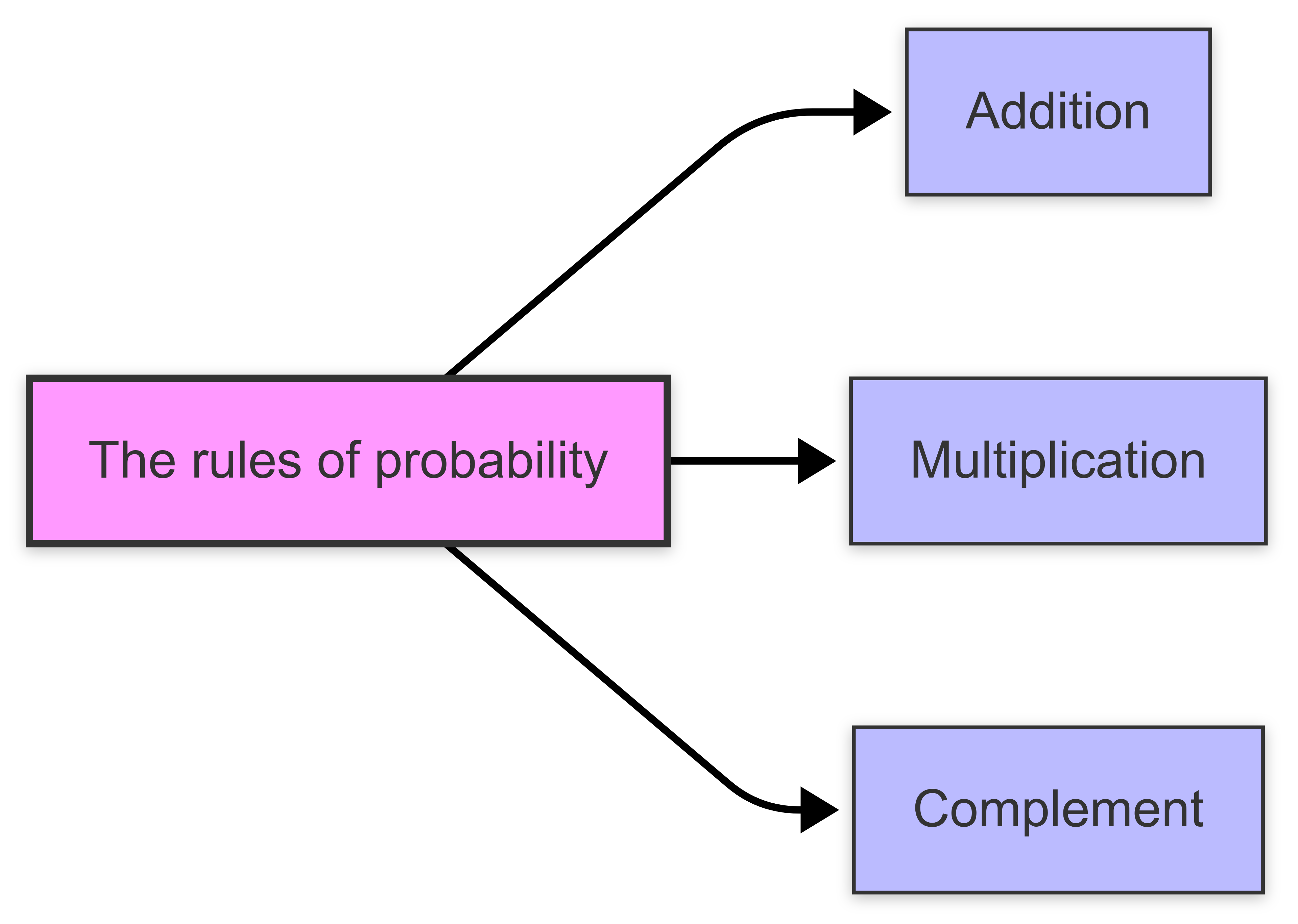
Introduction
In probability theory, several basic rules are used to calculate and apply probabilities.
The addition rule helps us determine the chance of any one of several mutually exclusive events happening. “Mutually exclusive” means these events cannot occur at the same time.
- For example, when flipping a coin, either heads or tails can happen, but not both simultaneously. This rule simplifies the calculation in such cases. The same would apply when calculating the outcome of penalty kick in football; it will be a goal OR a non-goal…it can’t be both.
On the other hand, the multiplication rule is used when we deal with independent events, where the occurrence of one event does not affect the other. This rule allows us to calculate the likelihood of both events happening together.
- For instance, rolling a dice and flipping a coin at the same time are independent events; the outcome of one does not impact the other.
Lastly, the complement rule is useful for finding the probability of an event not occurring. This often simplifies calculations by focusing on the opposite outcome.
- For example, if we want to know the probability of not rolling a six on a dice, we can first calculate the chance of rolling a six and then subtract that number from 100% to find the probability of it not happening.
The addition rule
The Addition Rule explains how to calculate the probability of one event or another occurring.
If two events, A and B, are mutually exclusive - meaning they cannot happen at the same time - the probability of either event occurring is the sum of their individual probabilities, \(P(A∪B)\)\(=P(A)+P(B).\)
However, if the events overlap, we must subtract the probability of both events happening at the same time: \(P(A∪B)=P(A)+P(B)−P(A∩B)\).
This ensures that overlapping probabilities are not double-counted. When dealing with more than two events, the rule can be extended by systematically subtracting overlapping probabilities.
The addition rule deals with the probability of either one event OR another occurring. There are two versions:
- For mutually exclusive events: \(P(A ∨ B) = P(A) + P(B)\) [P(A OR B) = …..]
- For non-mutually exclusive events: \(P(A or B) = P(A) + P(B) - P(A ∧ B)\) […P(A AND B)
The second formula subtracts the intersection to avoid double-counting overlapping probabilities.
The multiplication rule
The Multiplication Rule helps calculate the probability of two events happening together.
This image illustrates how the probability of both events occurring (P(A∩B)) is calculated by multiplying the individual probabilities P(A) and P(B) when the events are independent.
This second diagram shows dependent events, where the probability of Event B is conditional on Event A occurring first. The final probability is calculated using the conditional probability formula.
Definition
For independent events - where the outcome of one event does not affect the other - the probability of both occurring is simply the product of their probabilities, \(P(A∩B)=P(A)⋅P(B)\).
However, when events are dependent, the probability of the second event depends on the first.
In such cases, the rule is modified to \(P(A∩B)=P(A)⋅P(B∣A)\), where \(P(B∣A)\) represents the conditional probability of B given A.
This version of the rule is crucial for calculating probabilities in sequences of events.
Summary
The multiplication rule concerns the probability of events occurring together (AND). Like the Addition Rule, there are two forms:
- For independent events: \(P(A and B) = P(A) × P(B)\)
- For dependent events: \(P(A and B) = P(A) × P(B|A)\)
Here, \(P(B|A)\) represents the conditional probability of B occurring given that A has occurred.
The complement rule
The Complement Rule simplifies problems by focusing on what does not happen.
The image above illustrates how the sample space (S) is divided into two mutually exclusive parts: the event A and its complement Ac. The sum of their probabilities must equal 1.
Definition
It states that the probability of an event not occurring, \(P(Ac)\), is equal to one minus the probability of the event occurring, \(P(Ac)=1−P(A)\).
This is especially useful when calculating \(P(A)\) directly is complex, but finding its complement is easier.
For example, instead of calculating the probability of rolling at least one six with a pair of dice, you can calculate the complement - the probability of rolling no sixes - and subtract it from one.
The complement rule ensures that the total probability of all outcomes equals one.
Further explanation
The complement rule states that the probability of an event not occurring is 1 minus the probability of it occurring, or:
\(P(¬ A) = 1 - P(A)\) [P(NOT A)….]
This follows from the fact that probabilities must sum to 1 across all possible outcomes.
2.5 Conditional Probability
Introduction
‘Conditional probability’ is a concept in probability theory that helps us understand how the probability of one event changes when we have information about another event.
Conditional probability measures the likelihood of an event given that another event has occurred. It refines probability based on additional information.
Example
Let’s imagine a basketball player has an 80% chance of scoring a free throw. The event of scoring the free throw (A) depends on the occurrence of a foul (B) that grants the opportunity to take the shot.
The conditional probability is expressed as:
\[ P(A \mid B) = \frac{\text{scoring free throw}}{\text{foul occurred}} = 0.8 \]
This probability only makes sense in the context of the foul occurring, as without the foul, there would be no opportunity for the free throw!
This is an example of \(P(A∣B)\), where the probability of A(scoring the free throw) is conditioned on B(the foul). You could read this as “A IF B”.
What are ‘conditional’ events?
Conditional events refer to situations where the probability of one event depends on the occurrence of another.
For example, sticking with basketball, consider these conditional events: The probability of a player making their second free throw given that they made their first free throw • The probability of a team winning given that they are leading at halftime
In both cases, the probability of the second event (making second free throw, winning the game) is influenced by the condition of the first event (making first free throw, leading at halftime).
Conditional probability
This conditional probability is denoted as \(P(A|B)\). It represents the probability of event A occurring given that event B has already occurred.
It’s calculated using the formula:
\[ P(A|B) = \frac{P(A \cap B)}{P(B)} \]
This relationship shows that conditional probabilities are derived from the joint probability of A and B (their intersection), divided by the probability of the given event B.
Conditional events are central to identifying whether events are independent or dependent. For independent events, the occurrence of one does not affect the probability of the other, meaning:
\[ P(A|B) = P(A) \]
For dependent events, however, the probability of one event changes based on the occurrence of the other.
Conditional probability is the foundation of many probability concepts, such as the Multiplication Rule for dependent events:
\[ P(A \cap B) = P(A|B) \cdot P(B) \]
It is also fundamental to Bayes’ Theorem, which allows us to reverse conditional probabilities using prior and likelihood information:
\[ P(B|A) = \frac{P(A|B) \cdot P(B)}{P(A)} \]
The law of ‘total probability’
The Law of Total Probability breaks down complex probabilities into simpler parts.
If the sample space is divided into distinct events (called a partition), the probability of another event A can be found by summing over these partitions. For example, if B₁, B₂, …, Bₙ partition the sample space:
\[ P(A) = \sum_{i=1}^n P(A \cap B_i) \]
This can also be written in a conditional form:
\[ P(A) = \sum_{i=1}^n P(A|B_i) \cdot P(B_i) \]
where P(A|B_i) is the probability of A given B_i.
This rule is especially useful in real-world problems where probabilities depend on different scenarios.
ELI5
The Law of Total Probability is a way to figure out the chance of something happening by looking at all the different ways it could happen.
Imagine you’re trying to figure out the probability of an event, but that event depends on a few different situations or conditions.
Suppose you’re deciding the chance it will rain tomorrow. You know there are two weather forecasts: one says “sunny” and one says “cloudy.” The chance of rain depends on these forecasts.
- If it’s sunny, there’s a 10% chance of rain.
- If it’s cloudy, there’s a 50% chance of rain.
Now, let’s also say there’s a 70% chance it will be sunny and a 30% chance it will be cloudy.
The Law of Total Probability says you combine these possibilities by looking at:
- The chance it rains if it’s sunny × the chance it’s sunny.
- PLUS the chance it rains if it’s cloudy × the chance it’s cloudy.
So, the total chance of rain = \((0.1 × 0.7) + (0.5 × 0.3) = 0.07 + 0.15\) = 22%.
You’re breaking the problem into smaller pieces, working them out, and adding them together to get the full picture.
Probability trees
A probability tree is a visual tool used to calculate the probabilities of different outcomes in a sequence of events.
It’s especially helpful when dealing with conditional probabilities, multiple events, or situations involving dependent and independent events.
This probability tree shows:
- Two events (A and B) with their respective probabilities
- Conditional probabilities for event B given whether A occurred or not
- All probabilities at each branch level sum to 1
To find the probability of specific outcomes, multiply the probabilities along the desired path. For example, the probability of both events A and B occurring is 0.6 × 0.3 = 0.18.
Description
A probability tree represents events as branches, with probabilities assigned to each branch, making calculations more structured and intuitive.
Each branch in a probability tree corresponds to an event or outcome, and the probability of the event is written along the branch. At each split, the total probability of all branches must add up to 1.
For example, if an event has two possible outcomes (e.g., heads or tails in a coin flip), the branches will show the probabilities P(Heads)=0.5P(Heads)=0.5 and P(Tails)=0.5P(Tails)=0.5.
Conditional probabilities are represented by subsequent branches. For instance, if the first event influences the second, the second set of branches shows probabilities conditioned on the first outcome. To find the probability of a sequence of events, we multiply the probabilities along the path of interest.
For example, if Event A occurs with a probability of \(P(A)\)and Event B occurs afterward with a conditional probability \(P(B∣A)\), the probability of both events occurring is \(P(A∩B)=P(A)⋅P(B∣A)\).
Probability trees also simplify calculations for complementary events and mutually exclusive scenarios, allowing you to visually map all possible outcomes and their respective probabilities. This method is particularly useful for solving problems involving multiple stages, such as drawing cards, rolling dice, or decision-making under uncertainty.
By following the branches, even complex probability calculations become clear and manageable.
2.6 Independence and Probability
Introduction
Two events are independent if the outcome of one does not affect the probability of the other.
An example of two independent events in football would be:
- Winning a Coin Toss Before a Football Match: The outcome of the coin toss (e.g., heads or tails) is entirely random and does not influence other events in the game.
- Scoring a Goal During the Match: The probability of a team scoring a goal is completely unaffected by the earlier coin toss result.
These events are independent because the outcome of one (the coin toss) has no effect on the probability of the other (scoring a goal).
Independence is key to simplifying complex probability problems.
Pairwise independence
‘Pairwise independence’ is a property of random variables.
It means that any two variables in a group are independent of each other, but this doesn’t guarantee that the whole group is independent when looked at together.
For example, if you have random variables X,Y, and Z:
- X and Y are independent.
- Y and Z are independent.
- X and Z are independent.
This is pairwise independence. However, the group of X,Y, and Z might still influence each other when considered together, meaning they are not fully independent.
Pairwise independence only applies to pairs of variables, while full (mutual) independence applies to all variables in the group.
Example
Think of a group of friends. Two of them might act independently when making plans, but when all three get together, their decisions might depend on each other.
That’s pairwise independence without full independence!
Joint independence
Joint independence occurs when multiple random variables are independent of each other, not just pairwise but collectively.
Specifically, random variables \(X₁, X₂, …, Xₙ\) are jointly independent if the joint probability of any combination of their values equals the product of their individual probabilities:
\[ P(X_1=x_1, X_2=x_2, \ldots, X_n=x_n) = P(X_1=x_1) \cdot P(X_2=x_2) \cdot \ldots \cdot P(X_n=x_n) \]
for all possible values of \(x₁, x₂, …, xₙ.\)
This condition is stricter than pairwise independence, which only requires that any two variables are independent.
Remember: pairwise independence does not guarantee joint independence among all combinations of variables.
Testing for dependency
Dependency testing is the process of determining whether two or more variables are dependent or independent. It assesses whether changes in one variable are associated with changes in another.
Key methods for dependency testing include:
- Correlation Analysis: Measures linear dependency between two variables (e.g., Pearson’s correlation coefficient).
- Chi-Square Test of Independence: Tests the independence of categorical variables by comparing observed and expected frequencies.
- Mutual Information: Evaluates dependency by quantifying shared information between variables, useful for non-linear relationships.
- Regression Analysis: Examines dependency by modeling one variable as a function of others.
- Hypothesis Testing: Formulates null and alternative hypotheses to test independence, often with a statistical threshold (e.g., p-value).
2.7 Bayes’ Theorem - Probability and New Information
Introduction
If you’re unfamiliar with Bayesian Theory, you should read this first.
Bayes’ Theorem calculates the probability of an event based on prior knowledge and new evidence. In other words, it updates beliefs in light of new data.
Formula
The theorem is expressed mathematically as:
\[ P(A|B) = \frac{P(B|A) \times P(A)}{P(B)} \]
Where:
- \(P(A|B)\) is the posterior probability - the probability of A given that B has occurred
- \(P(B|A)\) is the likelihood - the probability of B given that A is true
- \(P(A)\) is the prior probability of A
- \(P(B)\) is the probability of observing B
The power of Bayes’ Theorem lies in its ability to incorporate new evidence to update probability estimates.
Prior probability
‘Prior probability’ represents our initial belief about an event or hypothesis before considering new evidence.
For example, if we’re trying to diagnose whether a patient has a particular disease, the prior probability might be the general prevalence of that disease in the population - say 1% or P(H) = 0.01. This represents our best estimate of the probability before we conduct any specific tests or observe any symptoms for this patient.
Prior probability forms the starting point for Bayesian inference (which allows us to update our beliefs as new information becomes available).
This initial probability estimate, often denoted as P(H) for a hypothesis H, reflects our knowledge, assumptions, or historical data before observing new evidence.
In netball, prior probability could be used to estimate a team’s chances of winning before a match. For example, if Team A has won 80% of their previous matches this season, we might set \(P(TeamAWins) = 0.8\) as our prior probability. This represents our initial belief about Team A’s likelihood of winning before considering specific match-day factors like player injuries, weather conditions, or the specific opponent.
Posterior probability
‘Posterior probability’ represents the probability of an event occurring after taking into consideration new evidence or data.
It updates our prior beliefs about an event based on additional information.
For example, if we initially believe there’s a 30% chance of rain (prior probability), but then observe dark clouds (new evidence), we can update our belief to a higher probability of rain (posterior probability).
Unlike classical (frequentist) probability, which relies solely on the frequency of events, posterior probability combines prior knowledge with observed evidence to form a more complete understanding of probabilistic events.
This is particularly valuable in real-world applications where new information constantly emerges and decisions need to be updated accordingly.
Example
In Formula 1 racing, teams might constantly update their race strategy based on new information. For example, if a team initially estimates a 40% chance of their driver winning (prior probability), they might update this probability after new evidence emerges during the race.
Now, the posterior probability gets updated based on factors such as:
- Tire degradation rates during the race;
- Weather radar showing incoming rain;
- Competitor lap times; or
- Fuel consumption data.
This continuous updating of probabilities helps teams make crucial decisions about pit stops, tire choices, and race tactics.
The likelihood function
The likelihood function describes how well a statistical model explains observed data by measuring the probability of obtaining that data given different parameter values.
The likelihood function plays a crucial role in Bayesian statistics through Bayes’ theorem: \(P(θ|x) ∝ L(θ|x)P(θ)\), where \(P(θ|x)\) is the posterior probability, \(L(θ|x)\) is the likelihood function, and \(P(θ)\) is the prior probability distribution.
This relationship shows how the likelihood function helps update our prior beliefs about parameters to obtain posterior probabilities, which is the foundation of Bayesian inference.
The likelihood function
In mathematical terms, the likelihood function \(L(θ|x)\) represents the probability of observing data \(x\) given parameters \(θ\).
Unlike a probability function that treats the data as variable and parameters as fixed, the likelihood function treats the observed data as fixed and the parameters as variable.
Example
Consider a badminton player’s serve success rate. We can use the likelihood function to estimate their true serving ability (\(θ\), or ‘theta’) based on observed serve data (\(x\)).
For instance, if we observe a player make 8 successful serves out of 10 attempts:
\[ L(θ|x) = C(10,8) * θ^8 * (1-θ)^2 \]
where: \(θ\) = true serving ability (parameter) x = 8 successes out of 10 (observed data)
By evaluating this likelihood function for different values of \(θ\), we can determine which serving ability parameter best explains the observed performance. A \(θ\) value of 0.8 would have a higher likelihood than 0.5, suggesting the player is likely a skilled server.
This analysis could help coaches assess player abilities, track improvement over time, and make strategic decisions during matches.